Submuestrear (a veces) no es pecado.Ejemplo

Listening

En un post anterior comentaba que submuestrear si es pecado. En este post vengo a contar algo así como un contraejemplo a mi mismo. O más bien, podríamos decir aquello de “dónde no hay no se puede sacar”, ¿ o si?

Para ver esto usaré un dataset muy conocido que está disponible en Kaggle, el de credit card. El sábado echando unas cerves con mi amigo Francisco me contaba que a él le salía bien sin submuestrear incluso haciendo una regresión logística, pero a mi no. Veamos.

Credit card

El típico ejemplo de creditcard de kagle.

# pruebo esto de la funcińo use nueva en r base.

use(package = "pROC", c("roc", "auc"))
use(package = "yardstick", c("mn_log_loss_vec"))

creditcard <- data.table::fread(here::here("data/creditcard.csv"))  |>  as.data.frame()
creditcard$Class  <-  as.factor(creditcard$Class)

table(creditcard$Class)
#> 
#>      0      1 
#> 284315    492

skimr::skim(creditcard)

Data summary

Name	creditcard
Number of rows	284807
Number of columns	31
_______________________
Column type frequency:
factor	1
numeric	30
________________________
Group variables	None

Variable type: factor

skim_variable	n_missing	complete_rate	ordered	n_unique	top_counts
Class	0	1	FALSE	2	0: 284315, 1: 492

Variable type: numeric

skim_variable	n_missing	complete_rate	mean	sd	p0	p25	p50	p75	p100	hist
Time	0	1	94813.86	47488.15	0.00	54201.50	84692.00	139320.50	172792.00	▃▇▅▆▇
V1	0	1	0.00	1.96	-56.41	-0.92	0.02	1.32	2.45	▁▁▁▁▇
V2	0	1	0.00	1.65	-72.72	-0.60	0.07	0.80	22.06	▁▁▁▇▁
V3	0	1	0.00	1.52	-48.33	-0.89	0.18	1.03	9.38	▁▁▁▁▇
V4	0	1	0.00	1.42	-5.68	-0.85	-0.02	0.74	16.88	▂▇▁▁▁
V5	0	1	0.00	1.38	-113.74	-0.69	-0.05	0.61	34.80	▁▁▁▇▁
V6	0	1	0.00	1.33	-26.16	-0.77	-0.27	0.40	73.30	▁▇▁▁▁
V7	0	1	0.00	1.24	-43.56	-0.55	0.04	0.57	120.59	▁▇▁▁▁
V8	0	1	0.00	1.19	-73.22	-0.21	0.02	0.33	20.01	▁▁▁▇▁
V9	0	1	0.00	1.10	-13.43	-0.64	-0.05	0.60	15.59	▁▁▇▁▁
V10	0	1	0.00	1.09	-24.59	-0.54	-0.09	0.45	23.75	▁▁▇▁▁
V11	0	1	0.00	1.02	-4.80	-0.76	-0.03	0.74	12.02	▁▇▁▁▁
V12	0	1	0.00	1.00	-18.68	-0.41	0.14	0.62	7.85	▁▁▁▇▁
V13	0	1	0.00	1.00	-5.79	-0.65	-0.01	0.66	7.13	▁▃▇▁▁
V14	0	1	0.00	0.96	-19.21	-0.43	0.05	0.49	10.53	▁▁▁▇▁
V15	0	1	0.00	0.92	-4.50	-0.58	0.05	0.65	8.88	▁▇▂▁▁
V16	0	1	0.00	0.88	-14.13	-0.47	0.07	0.52	17.32	▁▁▇▁▁
V17	0	1	0.00	0.85	-25.16	-0.48	-0.07	0.40	9.25	▁▁▁▇▁
V18	0	1	0.00	0.84	-9.50	-0.50	0.00	0.50	5.04	▁▁▂▇▁
V19	0	1	0.00	0.81	-7.21	-0.46	0.00	0.46	5.59	▁▁▇▂▁
V20	0	1	0.00	0.77	-54.50	-0.21	-0.06	0.13	39.42	▁▁▇▁▁
V21	0	1	0.00	0.73	-34.83	-0.23	-0.03	0.19	27.20	▁▁▇▁▁
V22	0	1	0.00	0.73	-10.93	-0.54	0.01	0.53	10.50	▁▁▇▁▁
V23	0	1	0.00	0.62	-44.81	-0.16	-0.01	0.15	22.53	▁▁▁▇▁
V24	0	1	0.00	0.61	-2.84	-0.35	0.04	0.44	4.58	▁▇▆▁▁
V25	0	1	0.00	0.52	-10.30	-0.32	0.02	0.35	7.52	▁▁▇▂▁
V26	0	1	0.00	0.48	-2.60	-0.33	-0.05	0.24	3.52	▁▆▇▁▁
V27	0	1	0.00	0.40	-22.57	-0.07	0.00	0.09	31.61	▁▁▇▁▁
V28	0	1	0.00	0.33	-15.43	-0.05	0.01	0.08	33.85	▁▇▁▁▁
Amount	0	1	88.35	250.12	0.00	5.60	22.00	77.16	25691.16	▇▁▁▁▁

El dataset está muy desbalanceado.

id_train <- sample(1:nrow(creditcard), 140000)
id_test <- setdiff(1:nrow(creditcard), id_train)


train <- creditcard[id_train, ]
test <-  creditcard[id_test, ]

(t1 <- table(train$Class))
#> 
#>      0      1 
#> 139751    249
(t2 <- table(test$Class))
#> 
#>      0      1 
#> 144564    243

prop.table(t1)
#> 
#>           0           1 
#> 0.998221429 0.001778571
prop.table(t2)
#> 
#>           0           1 
#> 0.998321904 0.001678096

Modelos glm normal, con submuestreo y con pesos

Comparando los tres glms con unas pocas variables, submuestrear parece ser mejor

Modelo normal sin submuestrear

No uso la variable Time, ni me caliento la cabez en buscar interacciones (por el momento)

f1  <-  as.formula("Class ~ V1 + V2 + V3 + V4 + V5 +V6 + V7 + V8 + V9 + V10 + V11 + V12 +V13 +V14 + Amount")

glm1 <- glm(f1, family = binomial, data = train)

(roc_glm <- roc(test$Class, predict(glm1, newdata = test, type = "response")))
#> 
#> Call:
#> roc.default(response = test$Class, predictor = predict(glm1,     newdata = test, type = "response"))
#> 
#> Data: predict(glm1, newdata = test, type = "response") in 144564 controls (test$Class 0) < 243 cases (test$Class 1).
#> Area under the curve: 0.5



(logloss_glm <- mn_log_loss_vec(as.factor(test$Class), predict(glm1, newdata = test, type = "response"), event_level = "second"))
#> [1] 0.0604847

# logloss(ytrue, predict(glm1, newdata = test, type = "response"))

Modelo glm submuestreado

Vamos a submuestrear la clase 0, pero no demasiado, nos quedamos con 3000

samples_0  <-  train[sample(rownames(train[train$Class == "0",]), 3000),]

table(samples_0$Class)
#> 
#>    0    1 
#> 3000    0

train_subsample  <- rbind(samples_0, train[train$Class=="1", ])
    
table(train_subsample$Class)
#> 
#>    0    1 
#> 3000  249

glm2  <-  glm(f1, family = binomial, data = train_subsample)

(roc_glm_submuestreo <- pROC::roc(test$Class, predict(glm2, newdata = test, type = "response")))
#> 
#> Call:
#> roc.default(response = test$Class, predictor = predict(glm2,     newdata = test, type = "response"))
#> 
#> Data: predict(glm2, newdata = test, type = "response") in 144564 controls (test$Class 0) < 243 cases (test$Class 1).
#> Area under the curve: 0.5546

(logloss_glm_submuestreo <- mn_log_loss_vec(as.factor(test$Class), predict(glm2, newdata = test, type = "response"), event_level = "second"))
#> [1] 0.2523929

Y en este caso , submuestrear parece ser mejor.

Modelo glm con pesos

# Pesos inversamente proporcionales al tamaño de la clase
pesos <- ifelse(train$Class == "1", sum(train$Class == "0")/sum(train$Class == "1"), 1)

# Modelo con pesos
glm_pesos <- glm(f1, family = binomial, data = train, weights = pesos)

(roc_glm_pesos <- pROC::roc(test$Class, predict(glm_pesos, newdata = test, type = "response")))
#> 
#> Call:
#> roc.default(response = test$Class, predictor = predict(glm_pesos,     newdata = test, type = "response"))
#> 
#> Data: predict(glm_pesos, newdata = test, type = "response") in 144564 controls (test$Class 0) < 243 cases (test$Class 1).
#> Area under the curve: 0.5

(logloss_glm_pesos<- mn_log_loss_vec(as.factor(test$Class), predict(glm_pesos, newdata = test, type = "response"), event_level = "second"))
#> [1] 35.98317

Y vemos que una regresión logística al uso no es suficiente para pillar hacer un modelo, en este caso submuestrear no es pecado, y no se ha arreglado usando pesos.

¿Pero y si usamos cosas de esas modernas, como los boosting?

Al Boosting

A ver qué pasa

Boosting tal cual

library(xgboost)


vars <- c("V1", "V2", "V3", "V4", "V5", "V6", "V7", "V8", "V9", "V10", "V11", "Amount")


# Preparamos las matrices
dtrain <- xgb.DMatrix(data = as.matrix(train[, vars]), label = as.numeric(as.character(train$Class)))
dtest  <- xgb.DMatrix(data = as.matrix(test[, vars]),  label = as.numeric(as.character(test$Class)))

# Entrenamos
xgb1 <- xgboost(data = dtrain, nrounds = 100, objective = "binary:logistic", verbose = 0)

# AUC
(roc_xg_boost <- pROC::roc(test$Class, predict(xgb1, dtest)))
#> 
#> Call:
#> roc.default(response = test$Class, predictor = predict(xgb1,     dtest))
#> 
#> Data: predict(xgb1, dtest) in 144564 controls (test$Class 0) < 243 cases (test$Class 1).
#> Area under the curve: 0.9617


(logloss_xgb<- mn_log_loss_vec(as.factor(test$Class), predict(xgb1, newdata = dtest), event_level = "second"))
#> [1] 0.003468277

Vaya, pues el boosting lo hace muy bien, al fin y al cabo son árboles encadenados, y pilla bien las interacciones

Boosting submuestreando

samples_0  <- train[sample(rownames(train[train$Class == "0",]), sum(train$Class == "1")), ]
train_sub <- rbind(samples_0, train[train$Class == "1", ])

dtrain_sub <- xgb.DMatrix(data = as.matrix(train_sub[, vars]), label = as.numeric(as.character(train_sub$Class)))

xgb2 <- xgboost(data = dtrain_sub, nrounds = 100, objective = "binary:logistic", verbose = 0)

# AUC
(roc_xgb_submues <- pROC::roc(test$Class, predict(xgb2, dtest)))
#> 
#> Call:
#> roc.default(response = test$Class, predictor = predict(xgb2,     dtest))
#> 
#> Data: predict(xgb2, dtest) in 144564 controls (test$Class 0) < 243 cases (test$Class 1).
#> Area under the curve: 0.9653

(logloss_xgb_submues<- mn_log_loss_vec(as.factor(test$Class), predict(xgb2, newdata = dtest), event_level = "second"))
#> [1] 0.163512

Boosting con pesos

# Calcular el ratio de clases
ratio <- sum(train$Class == "0") / sum(train$Class == "1")

# Entrenamiento con pesos
xgb3 <- xgboost(data = dtrain, nrounds = 100, objective = "binary:logistic",
                scale_pos_weight = ratio, verbose = 0)

(roc_xgb_pesox <- pROC::roc(test$Class, predict(xgb3, dtest)))
#> 
#> Call:
#> roc.default(response = test$Class, predictor = predict(xgb3,     dtest))
#> 
#> Data: predict(xgb3, dtest) in 144564 controls (test$Class 0) < 243 cases (test$Class 1).
#> Area under the curve: 0.9642

(logloss_xgb_pesos <- mn_log_loss_vec(as.factor(test$Class), predict(xgb3, newdata = dtest), event_level = "second"))
#> [1] 0.003572369

Pues los xgboost funcionan bien sea como sea.

Bayesiano

Y si hacemos una regresión logística bayesiana, pero poniendo como prior del intercept lo observado en los datos

# ponemos como prior el logit de la prevalenciaº

prop.table(table(train$Class))
#> 
#>           0           1 
#> 0.998221429 0.001778571

qlogis(0.0017)  # ≈ -6.38
#> [1] -6.375426
options(brms.backend = "cmdstanr")

library(brms)
f_hs <- bf(Class ~ V1 + V2 + V3 + V4 + V5 + V6 + V7 + V8 + V9 + V10 + V11 +V12 +
                    V13 + V14 + Amount)




prior_hs <- c(
  set_prior("horseshoe(2)", class = "b"),                # regularización para coeficientes
  set_prior("normal(-6.4, 2)", class = "Intercept")      # prior centrado en la prevalencia
)

El modelo full bayesian tarda bastante en Stan (tengo que poner el código en numpyro). ASí que cuando terminó de ajustarse lo guardé en un objeto serializado que luego llamaré

modelo_brm <- brm(
  f_hs,
  data = train,
  family = bernoulli(link = "logit"),
  prior = prior_hs,
  algorithm = "sampling",
  file = "modelo_brm_1",
  file_refit = "on_change",
  chains = 6, iter = 4000, cores = 6,
  backend = "cmdstanr"
)

Puedo hacer inferencia variacional para ver por dónde van los tiros

modelo_brm_vi <- brm(
  f_hs,
  data = train,
  family = bernoulli(link = "logit"),
  prior = prior_hs,
  algorithm = "meanfield",
  chains = 6, iter = 4000, cores = 6, 
  backend = "cmdstanr"
)
#> ------------------------------------------------------------ 
#> EXPERIMENTAL ALGORITHM: 
#>   This procedure has not been thoroughly tested and may be unstable 
#>   or buggy. The interface is subject to change. 
#> ------------------------------------------------------------ 
#> Gradient evaluation took 0.005593 seconds 
#> 1000 transitions using 10 leapfrog steps per transition would take 55.93 seconds. 
#> Adjust your expectations accordingly! 
#> Begin eta adaptation. 
#> Iteration:   1 / 250 [  0%]  (Adaptation) 
#> Iteration:  50 / 250 [ 20%]  (Adaptation) 
#> Iteration: 100 / 250 [ 40%]  (Adaptation) 
#> Iteration: 150 / 250 [ 60%]  (Adaptation) 
#> Iteration: 200 / 250 [ 80%]  (Adaptation) 
#> Success! Found best value [eta = 1] earlier than expected. 
#> Begin stochastic gradient ascent. 
#>   iter             ELBO   delta_ELBO_mean   delta_ELBO_med   notes  
#>    100        -1145.629             1.000            1.000 
#>    200         -777.796             0.736            1.000 
#>    300         -711.459             0.522            0.473 
#>    400         -698.357             0.396            0.473 
#>    500         -692.432             0.148            0.093 
#>    600         -697.675             0.032            0.019 
#>    700         -689.003             0.012            0.013 
#>    800         -698.835             0.011            0.013 
#>    900         -683.979             0.014            0.014 
#>   1000         -708.684             0.021            0.022 
#>   1100         -687.713             0.025            0.030 
#>   1200         -685.163             0.023            0.030 
#>   1300         -684.128             0.018            0.030 
#>   1400         -689.093             0.011            0.007   MEDIAN ELBO CONVERGED 
#> Drawing a sample of size 1000 from the approximate posterior...  
#> COMPLETED. 
#> Finished in  15.9 seconds.

summary(modelo_brm_vi)
#>  Family: bernoulli 
#>   Links: mu = logit 
#> Formula: Class ~ V1 + V2 + V3 + V4 + V5 + V6 + V7 + V8 + V9 + V10 + V11 + V12 + V13 + V14 + Amount 
#>    Data: train (Number of observations: 140000) 
#>   Draws: 1 chains, each with iter = 1000; warmup = 0; thin = 1;
#>          total post-warmup draws = 1000
#> 
#> Regression Coefficients:
#>           Estimate Est.Error l-95% CI u-95% CI Rhat Bulk_ESS Tail_ESS
#> Intercept    -8.09      0.11    -8.28    -7.87 1.00     1036     1069
#> V1           -0.00      0.01    -0.03     0.03 1.00      911      840
#> V2           -0.00      0.02    -0.04     0.03 1.00     1013      880
#> V3            0.01      0.02    -0.01     0.05 1.00      908      847
#> V4            0.48      0.05     0.39     0.57 1.00      651      883
#> V5            0.00      0.02    -0.03     0.04 1.00     1037      927
#> V6           -0.01      0.04    -0.10     0.06 1.00      954      941
#> V7           -0.02      0.03    -0.08     0.00 1.00     1018      982
#> V8           -0.14      0.04    -0.22    -0.08 1.00      862      980
#> V9           -0.01      0.04    -0.10     0.05 1.00      959      819
#> V10          -0.43      0.06    -0.55    -0.32 1.00      964      881
#> V11           0.00      0.03    -0.03     0.06 1.00      696      749
#> V12          -0.32      0.07    -0.45    -0.20 1.00      906      936
#> V13          -0.01      0.06    -0.10     0.03 1.00      902      906
#> V14          -0.62      0.05    -0.71    -0.53 1.00     1036     1026
#> Amount       -0.00      0.00    -0.00     0.00 1.00     1064      854
#> 
#> Draws were sampled using variational(meanfield).

Y como tenía entrenado y guardado el modelo full bayesian, lo puedo comparar

modelo_brm <- readRDS(here::here("modelo_brm_1.rds"))

summary(modelo_brm)
#>  Family: bernoulli 
#>   Links: mu = logit 
#> Formula: Class ~ V1 + V2 + V3 + V4 + V5 + V6 + V7 + V8 + V9 + V10 + V11 + V12 + V13 + V14 + Amount 
#>    Data: train (Number of observations: 140000) 
#>   Draws: 6 chains, each with iter = 4000; warmup = 2000; thin = 1;
#>          total post-warmup draws = 12000
#> 
#> Regression Coefficients:
#>           Estimate Est.Error l-95% CI u-95% CI Rhat Bulk_ESS Tail_ESS
#> Intercept    -8.27      0.16    -8.60    -7.97 1.00     2918     3039
#> V1           -0.01      0.03    -0.08     0.06 1.00     3223     6394
#> V2            0.03      0.04    -0.03     0.11 1.00     2950     4569
#> V3            0.11      0.06     0.01     0.22 1.00     1856     2353
#> V4            0.57      0.08     0.42     0.72 1.00     2404     3182
#> V5           -0.01      0.04    -0.11     0.07 1.00     3601     7578
#> V6           -0.01      0.06    -0.14     0.11 1.00     4277     5533
#> V7           -0.03      0.04    -0.13     0.04 1.00     4643     8040
#> V8           -0.16      0.03    -0.22    -0.10 1.00     5633     7150
#> V9            0.03      0.08    -0.11     0.21 1.00     1992     2599
#> V10          -0.50      0.09    -0.69    -0.34 1.00     3919     4417
#> V11           0.14      0.10    -0.02     0.34 1.00     2960     3591
#> V12          -0.12      0.08    -0.29     0.02 1.00     3063     3307
#> V13          -0.10      0.10    -0.31     0.04 1.00     3513     6012
#> V14          -0.66      0.07    -0.80    -0.52 1.00     2768     5983
#> Amount       -0.00      0.00    -0.00     0.00 1.00     5324     9345
#> 
#> Draws were sampled using sample(hmc). For each parameter, Bulk_ESS
#> and Tail_ESS are effective sample size measures, and Rhat is the potential
#> scale reduction factor on split chains (at convergence, Rhat = 1).

Y para calcular el roc auc hago la predicción de la media condicianada para cada observación.

probs_brm <- posterior_epred(modelo_brm_vi, newdata = test, ndraws = 1000)  |>  colMeans()

y_true  <-  test$Class

(roc_brm <- roc(y_true, probs_brm))
#> 
#> Call:
#> roc.default(response = y_true, predictor = probs_brm)
#> 
#> Data: probs_brm in 144564 controls (y_true 0) < 243 cases (y_true 1).
#> Area under the curve: 0.9744

Y el modelo bayesiano sin submuestrear con prior sobre el intercept funciona igual de bien que los xgboost, y es más interpretable.

Una cosa que nos permite el modelo bayesiano es obtener la incertidumbre de las predicciones. No la predicción de la media condicionada, sino la de cada observación, en esa predicción se le añade la incertidumbre debida a la distribución de los datos.

No es lo correcto para evaluar el modelo via auc_roc, pero podemos ver que sale

probs_brm_noise <- predict(modelo_brm, newdata = test, type = "response",ndraws = 1000)[, "Estimate"]

(roc_brm_noise <- roc(y_true, probs_brm_noise))
#> 
#> Call:
#> roc.default(response = y_true, predictor = probs_brm_noise)
#> 
#> Data: probs_brm_noise in 144564 controls (y_true 0) < 243 cases (y_true 1).
#> Area under the curve: 0.9384

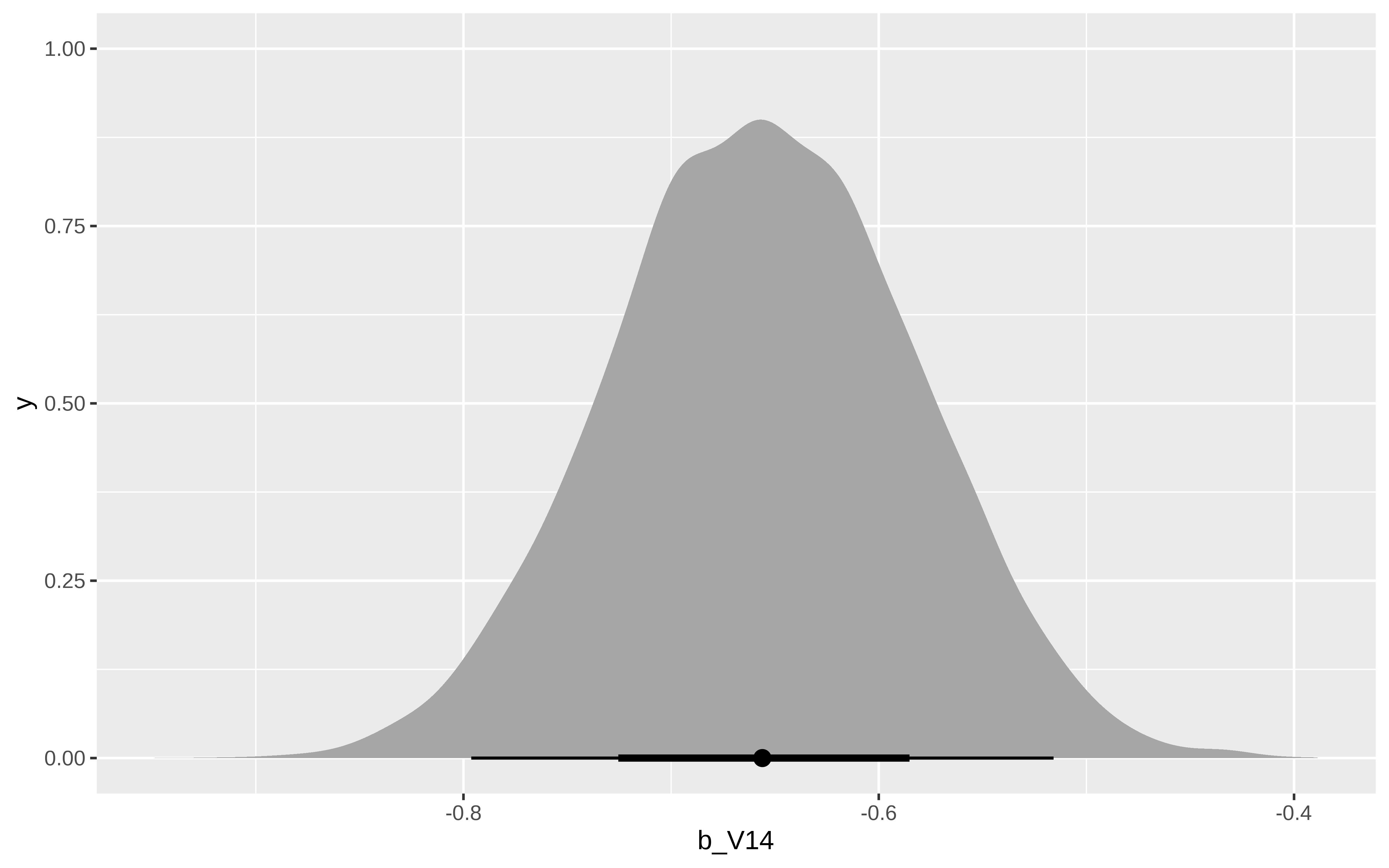
Podemos ordenar las variables por su coeficiente, por ejemplo

library(tidyverse)
coefs <- as_draws_df(modelo_brm)

# Extraemos solo las betas (coeficientes, no el intercepto ni parámetros auxiliares)
betas <- coefs %>%
  select(starts_with("b_")) %>%
  pivot_longer(cols = everything(), names_to = "term", values_to = "value")

# Calculamos media y percentiles
(summary_betas <- betas %>%
  group_by(term) %>%
  summarise(
    mean = mean(value),
    q025 = quantile(value, 0.025),
    q975 = quantile(value, 0.975)
  ) %>%
  arrange(desc(abs(mean))))  # ordenamos por magnitud de efectojj
#> # A tibble: 16 × 4
#>    term              mean      q025      q975
#>    <chr>            <dbl>     <dbl>     <dbl>
#>  1 b_Intercept -8.27      -8.60     -7.97    
#>  2 b_V14       -0.656     -0.796    -0.516   
#>  3 b_V4         0.570      0.424     0.719   
#>  4 b_V10       -0.505     -0.686    -0.344   
#>  5 b_V8        -0.162     -0.222    -0.0979  
#>  6 b_V11        0.143     -0.0200    0.343   
#>  7 b_V12       -0.122     -0.285     0.0171  
#>  8 b_V3         0.113      0.00727   0.224   
#>  9 b_V13       -0.103     -0.310     0.0413  
#> 10 b_V7        -0.0312    -0.125     0.0423  
#> 11 b_V9         0.0300    -0.113     0.214   
#> 12 b_V2         0.0257    -0.0344    0.111   
#> 13 b_V5        -0.0129    -0.109     0.0692  
#> 14 b_V6        -0.00752   -0.138     0.108   
#> 15 b_V1        -0.00593   -0.0767    0.0574  
#> 16 b_Amount    -0.0000297 -0.000462  0.000405


modelo_brm |> 
  tidybayes::spread_draws(b_V14) |> 
   ggplot(aes( x = b_V14)) +
  tidybayes::stat_halfeye()

Coda

A veces que esté muy desbalanceado el conjunto de datos hace que modelos sencillos como una regresión logística no funcione del todo bien, (hay mucho ruido en los 0’s). Otros modelos más complejos parecen funcionar bien, tanto sobre los datos originales, submuestreados o usando pesos. Pero dando un paso atrás y pensando en restringir el intercept de un modelo usando la prevalencia podemos ajustar un modelo bayesiano simple e interpretable y que funciona casi igual que esos modelos más complejos, y utilizando toda la información disponible. Curioso cuánto menos.